Utilizing Assimilated Whale Optimization and Deep Q-Learning to Interfere with Sensed Input Classification Model for Remote Patient Monitoring
Sayyed Johar* and GR Manjula
Published Date: 2025-03-21Sayyed Johar1* and GR Manjula2
1Department of Artificial Intelligence and Machine Learning (AIML), JNNCE-Shivamogga, Visveswaraya Technological University, Belagavi, Karnataka,
India
2Department of Computer Science and Systems Engineering, JNNCE-Shivamogga, Visveswaraya Technological University, Belagavi, Karnataka, India
- *Corresponding Author:
- Sayyed Johar
Department of Artificial Intelligence and Machine Learning (AIML), JNNCE-Shivamogga, Visveswaraya Technological University, Belagavi, Karnataka, India
E-mail:sayyedjohar@outlook.com
Received date: January 08, 2024, Manuscript No. IPMCR-24-18544; Editor assigned date: January 11, 2024, PreQC No. IPMCR-24-18544 (PQ); Reviewed date: January 25, 2024, QC No. IPMCR-24-18544; Revised date: March 14, 2025, Manuscript No. IPMCR-24-18544 (R); Published date: March 21, 2025, DOI: 10.36648/2471-299X.11.1.78
Citation: Johar S, Manjula GR (2025) Utilizing Assimilated Whale Optimization and Deep Q-Learning to Interfere with Sensed Input Classification Model for Remote Patient Monitoring. Med Clin Rev Vol:11 No:1
Abstract
Remote Patient Monitoring (RPM) systems, which are based on the Internet of Medical Things (IoMT), offer real-time data and insights on patients' illnesses without requiring frequent in-person visits to healthcare facilities. The wearable sensors are in charge of measuring people's psychological vitals at various intervals in order to determine their exact health state. In order to solve the continuous and discrete data extraction problems in RPM, this paper presents the Interfering Input Classification Model (IICM). The suggested approach combines deep-Q learning with whale optimization to identify connections and classify various interval data. The whales' search process ending is used to separate the felt data into discrete and continuous categories. The maximal discreteness of such classed data is verified, as is its relationship to earlier sequences. Using continuous clinical range correlations and Q-learning based on various state changes, this connectivity is carried out. The suggested model serves as an example of continuous and discrete signals, or data, for the purpose of anomaly identification and diagnosis suggestion. As a result, the suggested model may consistently increase accuracy and the classification ratio while introducing less errors.
Keywords
IoMT; Patient health monitoring; Q-learning; Sequence classification; Whale optimization
Introduction
The inability of modern hospitals to effectively monitor the health problems of numerous patients is one of their main issues. A different monitoring system for every patient is unproductive and less user-friendly when a major hospital has many patients that need to be watched at once [1]. A method or process that allows healthcare personnel to update patients' well-being and observe their state at all times is required. Consequently, IoMT (Internet of Medical Things) is a type of healthcare monitoring system that can efficiently send data for analysis and diagnosis [2]. Drug safety monitoring has become more transparent and clinical workflow management hasbecome easier because of the interconnection of medical equipment and sensors [3]. IoMT-based systems for evaluating patients remotely can improve the tracking and prevention of chronic illnesses and lead to more precise diagnoses [4]. IoMT applications enhance the healthcare system, as well as an examination of the state of implementations showing IoMT benefits to patients and the healthcare system [5]. Using a brief overview of the technology support, IoMT addresses the difficulties in creating a smart healthcare system [6].
Systems for diagnosing and monitoring healthcare facilities frequently incorporate data from wearable sensors. The process of moving data from one digital device to another is called data transmission [7]. The method of diagnosing medical conditions uses data from pre-processing, data segmentation, extraction of salient and discriminative features, and classification of activity [8]. Such analytical phases come before the actual data collection phase in human activity recognition, which uses a variety of sensors installed in mobile phones and wearable devices [9]. Pre-processing entails removing and presenting the unprocessed sensor data. To extract meaningful features, the segmentation technique splits the signal into many window widths [10]. In general, techniques such as sliding windows are used to separate sensor data. Feature selection techniques are frequently used to further limit the recovered features to the most discriminative characteristics for recognition tasks [11]. Statistical and structural aspects can be used to widely classify feature vectors for human activity recognition. While structural features leverage the relationships between the mobile sensor data to extract features, statistical features extract the quantitative qualities of the sensor data [12].
To monitor human health, Deep Learning (DL) a new area of machine learning that models high-level patterns in data is a significant trend. Multiple layers of neural networks used in DL hierarchically represent features, ranging from low to high levels [13]. More recently, several DL techniques have been put out for the detection of human behavior for sensors and mobile devices [14]. A thorough analysis of the latest advancements using deep learning-based human activity identification is performed using wearable and mobile sensors. DL-based human activity recognition exploits sensor data collected by mobile or wearable devices [15]. DL in time series includes voice recognition, sleep stage classification, and anomaly detection. To reduce classification mistakes and computational complexity, feature extraction helps to find lower groups from inputs. A suitable and efficient feature representation is necessary for the human health recognition system to function well. Consequently, the extraction of effective feature vectors from wearable and mobile sensor data aids in lowering computation times and producing accuracy [16,17]. The objectives of the article are listed below:
• To design an interfering input classification model using a Whale-optimized Deep-Q-Network (W-DQN) for detecting, classifying, and analyzing differentiation information from accumulated signals.
• To construct a data interconnection network that integrates continuous and discrete sensing sequences for error reduction and diagnosis improvements.
• To perform a wide assessment using external data and metrics to verify the efficacy of the proposed model.
Materials and Methods
Related works
Hou et al., developed a balanced signal preparation method with an adaptation technique for Machine Health Monitoring (MHM) [18]. The method suggests various Sparsity Measures (SMs) enhancements known as an Adaptive Weighted Signal Pre-processing Technique (AWSPT) to increase SMs' capabilities as Health Index (HI) for MHM. Theoretical quantities of AWSPT based SMs in healthy conditions are then looked at. The method selects the best envelope demodulation frequency band.
Meng et al., proposed a wearable convolutional neural network-based electrocardiogram signal monitoring and evaluation [19]. The number of network specifications was decreased and classification performance was enhanced by applying the cascaded small-scale kernel convolution. Some regularized techniques, like batch standardization. And dropouts were used to prevent overfitting. The suggested approach can improve wearable ECG data performance.
Wang et al., suggested a health index development using spatial monotonicity and sensor sparsity for mixed high dimensional signals [20]. Data fusion techniques are used to combine multi-sensor signals produced by the system into a scalar Health Index (HI). The approach develops a method for creating HI for picture and profile data called sparse group LASSO-principal component analysis. The method performs better than the benchmark methods.
Ding et al., introduced federated learning for the effective identification of epileptic seizures in the fog-assisted internet of medical things. The proposed Fed-ESD uses geographically distributed fog nodes as local aggregators to facilitate location based EEG signal exchange. A greedy strategy is presented for selecting the best fog node to serve as the coordinator node. The method is effective in terms of stability, scalability, and detection performance.
Jiang et al., developed a dispersive signal decomposition filter using iterative frequency-domain envelope-tracking approach. The recovered frequency envelope is then used to optimize GDs. The iterative processing mechanism is created to improve the TF resolution. An adaptive ridge detection technique is developed to automatically estimate the number of components. The method enhances the accuracy and efficiency of signal reconstruction.
Tasci et al., proposed an Electroencephalography (EEG) signal based dynamic patterns-based feature extraction tool for automatic identification of mental health. A unique collection of EEG signals was gathered from 69 people, comprising a control group and those with intellectual disability and bipolar disorder diagnoses. A new conditional feature extraction method extracts important features from the dataset. The approach offers compelling proof of the quantum local binary pattern's efficacy.
Shen et al., suggested a dynamic functional connectivity analysis and 3D convolutional neural networks to automatically identify Schizophrenia (ScZ). A cross-mutual information approach is presented for a time-frequency domain functional connectivity study to extract the features in each subject's alpha band. The suggested approach is tested using the public ScZ EEG dataset. The method improves the performance level of the method.
Wei et al., introduced directed EEG-based functional brain networks in the deception state. The method looked into the crucial neural networks that interact with brain information during deception. This investigation offers fresh viewpoints regarding the basic brain processes. The method provides compelling evidence for the evolution of brain networks.
Lee et al., developed a bio-signal monitoring clothes system for respiratory and ECG signal acquisition. The smart device's software platform offers actual time bio-signal observing and analysis of health data. The MIT/BIH arrhythmia information bases are used to confirm the good performance of the ECG QRS complicated recognition method. The method increases the sensitivity and positive prediction.
Xu et al., proposed an EHG signal analysis that employs network theory and its use in preterm prediction. Time Fourier Transform (STFT) is used to enlarge the initial signal in the time frequency domain. The suggested feature extraction technique is used to learn classifiers using EHG signals from the Term Preterm EHG database (TPEHG). The proposed method enhances the performance of sensitivity, specificity, overall accuracy, and AUC values.
Boll et al., suggested an artificial production of Vibroacoustic Modulation (VAM) signals for assessing structural health. Simple probe measurements are obtained at two stress levels of the structure when a steady state is established. The goal of the method is to pave the way for the eventual application of VAM to evaluate the structural soundness of intricate systems. The method lowers the sensor nodes' sensing needs.
Dang et al., introduced a data-driven systemic health tracking through feature fusion. The hybrid deep learning DCNN-LSTM architecture is predicated on the ability of the Convolutional Neural Network (CNN) to extract local information. The notable capability of the Long-Short-Term Memory (LSTM) network is used to learn long-term dependencies. The suggested approach produces a very accurate damage evaluation, comparable in accuracy.
Idrees et al., developed a lossless EEG data compression with epileptic seizure detection in IoMT networks. The Naive Bayes (NB) method is used to determine the patient's epileptic seizure status at the fog gateway. The same lossless compression algorithm from the first stage is used to lower the size of IoMT EEG data supplied to the cloud. The developed method beats the other approaches in terms of accuracy and offering high accuracy.
Proposed Interfering Input Classification Model (IICM)
The intelligent whale optimization is proposed to detect patient information from the wearable sensor. IoMT is used to monitor patient information at a different frequency. Here, pathological information is acquired from the patient, and classification and detection are performed. The detection is done by determining the patient's monitoring frequently for every instant of time. The wearable sensor is used to detect the heartbeat, pulse, and blood pressure. From the acquired sensor, the clinical data is forwarded to the database, where the interference and loss are addressed. The interference and loss are due to the frequency measure that took place during the sensing time. If the frequency sensing the device is longer than, the clinical data is fed into the system at a delay time. An illustration of the proposed IIC model is presented in Figure 1.

Figure 1: Illustration of IIC model.
To ensure the frequency for every instant whale optimization is used to classify the sequential and discrete data. This measurement is used to enroll the patient's daily value and monitor according to the fixed frequency which is at the limit. Thus, the computation is carried out for the detection and analysis of the signal from the wearable device. The data is forwarded to the clinical database where the mapping is done with the previous frequency range limit. In this case, Whale Optimization is used to classify the data and check for the iteration and update in the data. The best solution is attended until it reaches the maximum discreteness in the result. Thefollowing equation is used to recognize the wearable sensor signal that is being acquired.

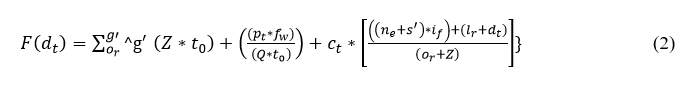
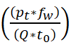
In the above Equation (1), recognition is done for the wearable sensor and deploys better sensing in the patients. Here, the signal is fed to the clinical database by sensing the data in the calculated frequency. In between the frequency limit the data signal is sensed and forwarded to the database. From this database, the computation takes place between the sensor and the database. The frequency range is measured for the iteration of the result that deploys the classification of sequential and discreteness. The continuous data is fed from the wearable sensor and forwarded at a particular time. From the particular time, the signals are acquired from the device on the preferred time limit. The sensor is used to regularly monitor the sensed data and analyze the result with the previously acquired result. This analysis takes place from the clinical database that addresses the interference and loss and it is represented as if and s'. The evaluation takes place by determining the signal from the sensor and it is described as g' and or. Thus, the recognition in Equation (1) is symbolized as Z, from this data is sensed and it is signified as ne. The data is sensed from the sensor to evaluate the recognition and it is observed as dt. Thus, the patient and the clinical database are symbolized as pt and ct, F is described as feeding the data into the database. The time is represented as t0, Q describes the frequency. Thus, the recognition is done from the wearable sensor, and the signal is acquired, post to this process the feed into the clinical system is based on time and frequency. The following equation is used to illustrate the clinical database which feeds the data from the sensor.
The sensed data is fed to the clinical database and deployed to address the interference and loss. A timely manner is followed to send the sensed data and find the loss. Here, the patient-sensed data is acquired from the sensor and provides the classification for the sequences and discrete data. The sequence and discrete data are acquired from the wearable devices and forwarded to the clinical center. If the timely manner is not followed then, the patient’s emergency case is attended. Thus, the evaluation takes the sensed data from the different frequency that holds the signal ranges for varying input from the sensor. In this case, the sensed data along with this frequency is measured and forwarded the data to the clinical center. The loss and interferences are addressed in this paper by introducing the whale optimization method.
The data is fed to the system that examines the signal from the patients and it is based on the frequency. The frequency is done for the different signals from the wearable sensor, and the forwarding is described as fw. Thus, the evaluation is done in different iterations along the frequency of the signal is also measured. A timely manner is followed for the data forwarding from the patients and it is represented as:
The signals from different patients with varying frequencies are calculated in the clinical center that states if there is any emergency case to attend. The emergency case is defined from the previous data history and mapping is performed with the current state of signal acquiring. For every set of iterations, the processing is carried out based on the clinical signal. From this time and frequency are measured from the data fed to the system, here interference and loss is addressed by using whale optimization.
Whale optimization
The optimization problem is addressed by using whale optimization, its mathematical process is to search for the prey, encircle the prey, and spiral bubble-net feeding. Based on these three processes whale optimization works, the initial stage is to search for the prey here is defined as sensing the clinical data. Then, comes encircling the prey, in this work, the signal sequences and discrete are analyzed and encircles the discrete data. The spiral bubble net-feeding states the number of iterations and updates in the sensed data and obtains the best discrete solution. Thus, the mechanism works in the whale optimization for patient monitoring, from this classification is determined by the following equation that categories are sequential and discrete.
In the above equation, whale optimization is used to classify the discrete and continuous. The recognition of the signal is forwarded to the clinical database. Here, the sensor feeds the signal, and iteration is processed based on the clinical database. The frequency of data is acquired and analysis is carried out to improve the discrete data. The classification is used to find the prey here it refers to the sensor data from which forwarding is carried out. Post to the sensor data prey searching the encircling is done for the different signals and exploring the frequency. The encircling is done by deploying the discrete data and providing the desired data. The evaluation is carried out in the frequency and estimate of the relationship between the violation and continuous signal. The processing is done by deploying the time and frequency which are fed to the clinical data. The whale optimization encircles the discrete data from which the signal is acquired and provides the result. The bubble-net is used to estimate the updating for the number of iterations. The classification process is described in Figure 2.

Figure 2: Classification process of β.
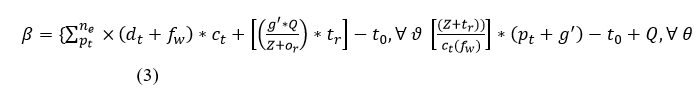
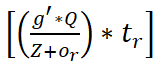
The classification is performed using Z input for ne extraction from dt. The whale agents are identified from the F (dt) defined intervals for verifying fw=true/false. In this case the ctand Pt updates are crucial across multiple s'. First, if fw=true then dt+1 is the search (classification) start-over point. The contrary Whale optimization The optimization problem is addressed by using whale optimization, its mathematical process is to search for the prey, encircle the prey, and spiral bubble-net feeding. Based on these three processes whale optimization works, the initial stage is to search for the prey here is defined as sensing the clinical data. Then, comes encircling the prey, in this work, the signal sequences and discrete are analyzed and encircles the discrete data. The spiral bubble net-feeding states the number of iterations and updates in the sensed data and obtains the best discrete solution. Thus, the mechanism works in the whale optimization for patient monitoring, from this classification is determined by the following equation that categories are sequential and discrete. In the above equation, whale optimization is used to classify the discrete and continuous. The recognition of the signal is forwarded to the clinical database. Here, the sensor feeds the signal, and iteration is processed based on the clinical database. The frequency of data is acquired and analysis is carried out to improve the discrete data. The classification is used to find the prey here it refers to the sensor data from which forwarding is carried out. Post to the sensor data prey searching the encircling is done for the different signals and exploring the frequency. The encircling is done by deploying the discrete data and providing the desired data. The evaluation is carried out in the frequency and estimate of the relationship between the violation and continuous signal. The processing is done by deploying the time and frequency which are fed to the clinical data. The whale optimization encircles the discrete data from which the signal is acquired and provides the result. The bubble-net is used to estimate the updating for the number of iterations. The classification process is described in Figure 2. 4 condition is the β initialization for v and θ for Pt and Ct classification. If de=Ne is satisfied the classification is terminated the if is identified and ne initialization is performed (Figure 2). Based on the iterations and updates the bubble-net mechanism is used in the Whale optimization. In Equation (3), classification is performed and it is represented as β, the first condition states the sequences whereas, the second condition describes the discrete and is symbolized as ϑ and θ. Thus, the computation is performed in this IoMT by using Whale optimization. The first case defines the sensing and forwarding to the clinical database and this is based on the number of iterations and is represented as:
So, the sequences of data are performed whereas, the second is processed based on the signal and frequency count. This evaluation process uses discrete data on different time intervals and it is described as (pt+g')-t0+Q. From this classification method, in whale optimization, the bubble-net mechanism is processed to find the violation and continuous signals. It is done by evaluating the iteration from the classification to perform the bubble-net mechanism. The following equation is used to evaluate the iterations from the classification method.
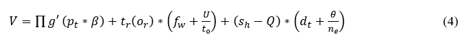
The evaluation has taken place for the sensed data and determines the better output based on the time and frequency. The frequency of data and the signal are examined from the recognition of data and provide the best data identification. At a particular time, the signals are acquired and processed to attain better recognition. The signals are acquired from the classification phase which includes the continuous and discrete data. Here, the computation step includes data identification, and frequency is observed for every interval of time. For every iteration, the frequency check is performed among the relationships between the continuous and discrete. The processing is done for the relationship between the violation and continuous signals and it is described as sh. Equation (4) includes the processing that deploys the discrete signal, which is sensed and it is represented as (dt+θ/ne). The bubble net in Whale optimization is used to provide the iteration and update for every step of the computation. The update is symbolized as U, this is carried out for every set of evaluation steps and it is described as V. Thus, the signal is acquired and examines the relationship between continuous and discrete signal processing. The frequency strength is evaluated to observe the better bubble-net mechanism by using iteration and update of discrete signals. Post to this evaluation method, the position sequences are established for the discrete and continuous signals and it is equated in the below equation as follows.
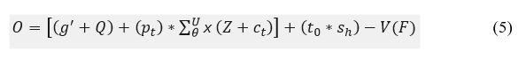
The observation is performed for the different set of signals that deploys the connection between the wearable sensor and the signal. The emergency case is analyzed based on the relationship between the violations and continuous in this continuous observation process. If the signal is transmitted to the clinical database, the mapping is performed with the current the previous history. The observation is represented as O, in which the analysis is carried out for every iteration and an update from the bubble-net of whale optimization. Thus, the frequency is analyzed, this is based on the update and recognition of signals and it is represented as:
The algorithmic representation of the classification process is given in Algorithm 1.
Algorithm 1 classification
Input: Z
Output: β
1: For all dt ∈ Z do
2: Compute F (dt) using Equation (2)
3: Perform fw for t=1 to n
4: if {dt=Ne} {then
5: Update dt=dt+1; fw ∈ ϑ
6: Else
7: Compute (pt+g') ∀ tr=True
8: Update Ct, Pt
8: End if
9: if {dt=dt+1} {then
10: Group: (dt-to) ∈ ϑ //Continuous
11: Else group: (Z+Q) ∈ θ //Discrete
12: End if
13: End For
The interconnection of the network is done to find the relationship between the violation and continuous data. The processing states the connection and estimates the iterations and updates. From this, the following equation is used to interconnect Equations (4) and (5).
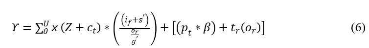
The interconnection is performed to find the best solution in the clinical data. This computation step feeds the signal to the database, and mapping is performed by observing the position sequences and iteration steps. For every instance of time, iteration and update are performed based on the relationship. The interconnection is represented as Υ, where the position of sequences is analyzed by using whale optimization. Thus, the evaluation is performed for the better iteration step that deploys the classification in this optimization. The verification is performed for the relationship of violation and continuous signal, and it is formulated in the below equation.
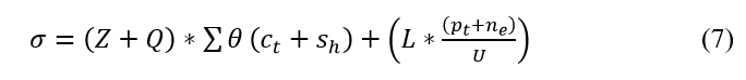
The verification is performed in the above equation and it is represented as σ. The process here is used to deploy the classification of sequence and continuity. Here, the relationship is defined for the varying position sequences and finds the violation, and it is symbolized as L. The discrete signals are acquired and perform better reliability for clinical data. The medical signal is given as the input and provides the update for every iteration step. The verification is done for every set of iterations and provides the frequency-based relationship which includes the violation and continuous signal. To avoid this maximum discreteness is identified in the following equation.
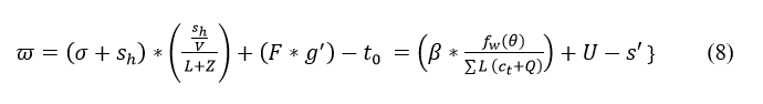
The verification is carried out in Equation (7), and from this identification is done for the sensor signal and forwarded to the clinical database. The processing is done for the frequency monitoring that acquires the iterations and updates and estimates the better computation. The verification is described as ϖ; in this signals are acquired and forward the emergency data to the clinical database. The iteration and position updates for extreme classification are presented in Figure 3. This is performed for maximum discreteness detection.

Figure 3: Iteration and position classification.
The maximum ne under varying dt is used for identifying sh and the first update is gathered for v=θ verification. If this case is true, then the condition for sequence violation is L from which the last known Z ∈ t is the continuous signal. Post this equal the intervals are discrete for which the position Pos=t and iteration for discreteness is incremented. In the failing case (i.e.) v>θ the violating is 0 (i.e.) no discreteness is identified. Therefore the position of Z is further verified for t=t+1 (i.e.) it is a continuous signal. If this fails, then γ is the discreteness and the maximum discreteness in Z ∈ dt is (L*θ). Otherwise, the sequence for continuous and discreteness is updated (Figure 3). The maximum discrete is identified in the above equation that provides the signal variation on time. The discrete signal is identified and analysis whether it provides the best solution. If the process does not acquire the maximum discreteness then the deep Q network is introduced to address this issue. The following section focuses on deep Q-network.
Results and Discussion
Deep Q-network
In the deep Q-network, the input is fed into the network, and in return, the Q-value provides the output. Here, the input is the medical data with discreteness which is processed from the Whale optimization. Post to this method, deep Q-network is introduced in this proposed work, in these two categories are done, one is normal and abnormal. Both the state is defined from the patient history and it is mapped to the previous and provides the result. The following equation is used to categorize the normal and abnormal signals from the medical signal.
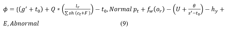
The deep Q-learning is introduced to produce the maximum discreteness which is identified in Equation (8). From this maximum discreteness is not achieved to improve this deep Q network is established by categorizing the normal and abnormal signals. Both signals are classified by the previous state of processing. The history of the medical signal is used to map the current and previous state and it is represented as hy. If there are any emergency case exits the mapping is done along with the frequency of the signal and it is described as E. Based on this computation step, normal and abnormal are categorized and it is symbolized as φ. For this deep Q-learning acquires theabnormal data as the input and performs the deep learning concept. From the deep learning concept, the output with the Q-value is returned to the center. The following equation is used to establish the connection for the discrete and abnormal signals.
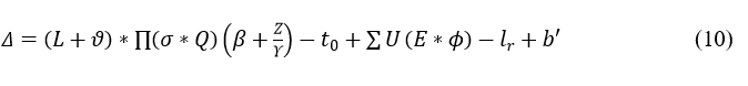
The connection is established between the clinical center and the wearable sensor. Here, the classification is done for the normal and abnormal data which is mapped with the previous state. The emergency case is observed in the abnormal signal in which the matching is performed. The connection is established by using a deep Q-network that deploys the discrete signal. The frequency range is monitored based on the classification model and it is represented as:
The establishment is done to avoid the violation and continuous signal, and it is described as Δ. The abnormal signal is symbolized as b', post to this method differentiation is done on the clinical data. The input is the abnormal data and from this output is the used to diagnose the patient.
The differentiate is done for the abnormal signal and provides the efficient result which is based on time. The frequency is established which forwards the signal to the clinical database that provides the position sequences. The position sequence is recognized for the categorized signal which involves abnormal signal. The Q-Learning for relating abnormal and normal sequences is presented in Figure 4.

Figure 4: Q-Learning for relating abnormal and normal sequences.
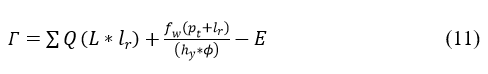
The state learning process is been in identifying Δ or fw based on ϖ and σ respectively. The Γ with E's influence for the discrete and continuous intervals are detected for (L-ϖ) improvement. This verifies the connectivity matching through further observation sequences for b^' (atleast) detection. If such occurrence is detected θ is matched with v from which v is identified. The case of σ (verification) of the accumulated data is pursued towards further diagnosis. The history of the signal in the database is represented as hy. The Differentiate is done as high and low which provides the output as a discrete diagnosis. Based on this discrete and diagnosis model, the clinical data is examined based on a timely manner. Here, Γ is represented as differentiating that deploys the discrete and diagnosis. From this higher value, a better diagnosis is pursued. To improve this process history of data is executed by performing matching, and it is formulated in the below equation.

In the above equation, a determination is made to analyze the abnormal state by performing mapping with the history of the signal. Here, the evaluation is done by deploying the normal and abnormal state of the patient and providing the result promptly. The identification is done to obtain the maximum discreteness. The matching for the connectivity verification process is presented in Figure 5.

Figure 5: Matching for connectivity verification.
The matching process is performed for Γ identified in Ne ∈ v sequences. The other sequence of θ is induced for variation and maximum differentiation outputs. On the contrary process of input signal assessment, both L and its corresponding θ to v verification need to coexist. Such cases are thus classified for normal and abnormal signals based on different intervals such that a history update is performed after to or E detection (Figure 5). The emergency state is defined for the abnormal patients and performs the mapping and it is represented as

Matching in this equation is symbolized as M. From this accuracy level is improved by the analysis method, and it is equated in the following equation.
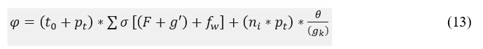
In the above Equation (13), the accuracy level is improved and diagnosis is done for the emergency patient in the initial stage. Here, the processing involves the signal forwarding to the center and monitoring the frequency in less time. The high rate of connection is said to be an emergency case and it is described asgk. The accuracy is represented as φ; in this patient daily monitoring and frequency count are calculated based on the deep Q-network. Thus, the proposed work satisfies the periodic patient monitoring for abnormal cases and addresses the inference and loss. The connectivity assessment process is presented as steps in Algorithm 2.
Algorithm 2 connectivity check
Input: θ
Output: Γ
1: For all dt ∈ hy do
2: Compute (φ) using Equation (9)
3: If {φ=g'} {then
4: Computer Δ using Equation 10; Update b'=0
5: Else if {φ=E} {then
6: Perform M using Equation (12)
7: if {M=max(x)} then
8: Update Δ=(L+ϑ); b'=0, ϑ=0
9: Update dt=dt+1; dt+1=0
10: Repeat from Step 6: until φ=g' and b'=0
11: Update Q+ct
12: End if
13: Perform algorithm 1
14: Compute Γ using Equation (11) ∀ ϑ=dt+1
15: End If
16: End For
Data-based assessment
The proposed model is correlated for its performance using the “multimodal stress dataset” provided. This dataset is created using wearable sensor data accumulated from 15 working people for 1 week. Using this data the stress level of the working people is identified; the classification of continuous or discrete is performed using the proposed IICM. For ease of understandability, the data and accumulation process are presented in Figure 6.

Figure 6: Data accumulation and interval representation.
The wearable sensor aggregates signals under 3 sensing intervals; low (0.25), normal (2-6), and abnormal (5-25). These observed/sensed signal data are classified as high/low for identifying stress. This stress detection is regarded as normal/ abnormal for health concerns. Therefore for the 4 signals above the v and θ variants are analyzed at an average for 15 sets of inputs in Figure 7.

Figure 7: v and θ variations for 4 signals.
For a maximum of 25 hours of signal observation, the v and θ variations are computed using fw and β processes. In the iteration-based assessment, if L is observed in any sensing interval, the ϖ at that instance is computed. This is required for computing the difference between successive intervals. If the difference is high then abnormality is observed and therefore diagnosis is required. Here the diagnosis refers to the stress identified and therefore the β process is repeated from the first Γ point. Say, for example, the change in heart rate is observed in 24 hrs, then the position is 24, and iteration is pursued independently from the 23rd hour. If this replication is seen anywhere further, then the difference between ranged clinical values and observed values are used for stress detection (Figure 7). In the pursuing analyses, the ϖ and Δ for the different iterations are analyzed. The analysis is presented in the below Figure 8.

Figure 8: ϖ and Δ analyses for different iterations.
The optimization-based classification requires verification failing and sequence discontinued intervals for ϖ estimation. In this process, the β ∈ v or β ∈ θ are the identifiable classifications for v under sh. This does not match with history and therefore clinical value correlation is performed. Hence the violating sequences (i.e.) v>θ is the iteration required instances and the previous observation interval requires σ. Thus the iterations focus on reducing ϖ such that Δ is improved (Figure 8). Finally the difference detection from the clinical value (range) for the 4 signal inputs is analyzed in Figure 9. This analysis is performed for the varying hours and working peoples.

Figure 9: Γ analysis for hrs and peoples.
The Γ variation is analyzed for the clinical range for both low and high observation intervals. In this variation analysis, the M is the steep process for maximizing v other than ϖ is induced for better outputs. The state analysis is pursued v or θ matching with the observed data and clinical history. Therefore the differentiation for φ=false condition is performed for reducing Γ. Hence the repeated iterations are pursued under (L, σ) ∈ M for this purpose from different sensing intervals (Figure 9).
Performance assessment
The performance assessment is validated using classification ratio, signal identification, classification accuracy, time, and error. The sensing intervals (15 s to 180 s) and input data (0.25 K to 2.5 K) are varied in this assessment. The methods DCNN LSTM, SGL-PCA, and HVG-FE are the methods accounted for from the related works section for the comparative study.
Classification ratio
The classification ratio for the proposed work increases in the clinical data for varying sensing intervals and input data and deploys the signal from the wearable sensor. Here, the normal and abnormal signals are detected for evaluating different iterations and updates. The recognition is done for the wearable sensor and acquires the signals and it is derived as:

The normal signals are omitted and abnormal signals are detected as emergency cases. The frequency is processed for every assigned interval and provides the signals from the sensor. The classification model is done by introducing Whale optimization that examines the continuous and discrete signals. The iteration and update are processed for the discrete signals.
The violation and continuous signals are addressed in this approach and estimate the better classification. The classification is equated in Equation (3) based on this iteration, and an update is performed. For every set of signals that are acquired from the wearable devices, the frequency is calculated for the periodic time. Thus, the classification ratio is the initial step for this proposed work, and the output is based on this discrete signal (Figure 10)

Figure 10: Classification ratio.
Signal identification
In Figure 11, the signal identification increases to find the maximum discreteness in the signals for different sensing intervals and data input. The processing step calculates the better reliability among the clinical center and the patients. If the patient signals are sensed, forwarding is done promptly. The sensing is measured with the current and the previous set of data and it is represented as
In this computation step, the inference and loss are addressed in this approach and derive the recognition of frequency and signals. The evaluation states the classification of the signal and provides the abnormal state. If the signal is abnormal, then, the categorization is performed for the relationship between the violation and continuous signals. If there is any violations are detected then, the identification is calculated for the maximum discreteness and it is formulated in Equation (8). This equation is used to state the discreteness of signals and provides the best detection of discreteness. Once the discreteness is classified then, the maximization is observed. By performing this, the signal identification is improved in this work.

Figure 11: Signal identification.
Classification accuracy
The classification accuracy shows better improvement for varying sensing intervals and data input. This is achieved by recognizing the signal whether it is normal or abnormal based on this Whale optimization is processed. The evaluation step is used for the detection of iteration and update. Both the iteration and update are done to enhance the accuracy level. If the accuracy level is improved then, the inferences and loss are reduced in the approach and it is equated as
The clumping of iteration and position sequences is estimated to find the best solution. The best solution is identified from the classification accuracy and provides the relationship between the discrete and continuous. The categorization is done in the normal and abnormal which address the signals with loss. The discrete signal is detected from the classification and shows a better accuracy rate and it is formulated as (fw+U/t0). Thus, for every step of processing update is performed by deploying the connection between the signals and frequency count. In this accuracy is calculated for every set of iteration and update in the proposed work (Figure 12).

Figure 12: Classification accuracy.
Classification time
In Figure 13, the classification time decreases for different sensing intervals and data input provides the iteration factor, and finds the best solution. The best solution is derived from the t ime and frequency range of the discrete signals. The relationship is estimated for the signal fed into the database that decreases the loss and it is represented as (t0 × sh)-V(F). The periodic monitoring is observed for the iteration and frequency and it is formulated as

The signals and frequency are used to address the inference and the loss from the sensor data and provide the best accuracy. The classification time for the proposed work describes the high and low connections. The Deep Q-network is used to estimate the sensing intervals and data input in the proposed work and provides a better classification. The classification time for the proposed work decreases by evaluating the maximum discreteness in the proposed work. Here, the patient history is analyzed by mapping the current and the previous set of processing. Thus, by computing this process the classification time for the proposed work decreases.
Figure 13: Classification time.
Error
The error in the proposed work is reduced for varying sensing intervals and data input. The error is addressed by combining Whale optimization and deep Q-network this states the best solution from the maximum discreteness. The relationship factor is estimated for the violation and continuous signals. The verification is performed for the different sets of intervals and times and it is formulated as
The update is done for every iteration step and provides the desirable output based on the differentiation of high and low connections. The emergency case is addressed in this proposed work and provides the treatment in the required time. A timely manner is done to evaluate the position sequences, and that diagnosis is performed. The performances are carried out for the different sets of interval and input data. The frequent references are estimated for the iteration and update and decrease the error rate. The frequency is monitored for the patient and diagnosis is made on time. By this computation, the error rate is decreased in the proposed work and shows better diagnosis (Figure 14). Table 1 presents the performance assessment summary for the different sensing intervals.

Figure 14: Error.
| Metrics | DCNN-LSTM | SGL-PCA | HVG-FE | INC-W-DQN | Findings |
| Classification ratio | 44.94 | 52.17 | 63.9 | 69.524 | 7.93% high |
| Signal identification (Interval) | 0.867 | 0.891 | 0.923 | 0.9569 | 6.32% high |
| Classification accuracy | 0.892 | 0.912 | 0.928 | 0.9423 | 9.49% high |
| Classification time (ms) | 904.31 | 692.7 | 519.22 | 235.715 | 11.1% less |
| Error | 0.104 | 0.091 | 0.079 | 0.0432 | 9.63% less |
Table 1: Performance assessment summary (Sensing intervals (s)).
The number of sensing intervals are varied from 15 to 150 s with 15 s difference. Such observation interval is modeled for different devices for sensing and forwarding data in a synchronized manner. The missing or inappropriate sensing interval is used for classification as sequence or discrete and then normal or abnormal. Based on this observation, the last observed comparative analysis value is tabulated in the Table 1. The summary for varying input data is presented in the Table 2.
| Metrics | DCNN-LSTM | SGL-PCA | HVG-FE | INC-W-DQN | Findings |
| Classification ratio | 47.5 | 55.99 | 64.79 | 69.393 | 6.65% high |
| Signal identification (interval) | 0.879 | 0.895 | 0.929 | 0.9573 | 6.63% high |
| Classification accuracy | 0.898 | 0.915 | 0.935 | 0.9496 | 10.08% high |
| Classification time (ms) | 900.82 | 687.15 | 541.64 | 304.86 | 9.51% less |
| Error | 0.109 | 0.083 | 0.081 | 0.0403 | 10.14% less |
Table 2: Performance assessment summary (Input data (K)).
Table 2 is distinct from the previous by considering the number of data records that are eligible for validation. The input data is nearly 4 observations per working person for 7 days for 100 days. This provides a cumulative of 2.8 K inputs from which 2.5 K is selected for the comparative analysis. Similar to the previous comparison, this variant also identifies the last observed value of the inputs.
Conclusion
This article introduced the interfering input classification method for improving the diagnosis accuracy of patients through remote health monitoring. The wearable sensors, computing devices, and storage are interlinked using the conventional IoMT. The sensed signals have definite intervals for accumulating and transmitting them using the IoMT communication medium for clinical analysis. In this model, the interfering discreteness between the consecutive sequences is classified using whale optimization. The position and iteration behavior of the whales are used for updating the discreteness instance for mitigation. In the Q-learning process, the classified sequences are correlated using external input data for matching. This matching is used to improve the classification accuracy over abnormal and normal sequences. The learning process recurrently analyzes the matching factor from the whale identified position (sequence). Based on the joint processes, the proposed model is distinguishable for identifying and classifying sequences from different sensed intervals. The proposed model improves accuracy by 9.49% and reduces error by 9.63% for the varying sensing intervals.
Conflict of Interest
The authors declare that they have no conflict of interest.
Funding
This research received no specific grant from any funding agency in the public, commercial, or not-for-profit sectors.
References
- Karolcik S, Ming DK, Yacoub S, Holmes AH, Georgiou P (2023) A multi-site, multi-wavelength ppg platform for continuous non-invasive health monitoring in hospital settings. IEEE Trans Biomed Circuits Syst 17:349-361
- Mao J, Zhou P, Wang X, Yao H, Liang L, et al. (2023) A health monitoring system based on flexible triboelectric sensors for intelligence medical internet of things and its applications in virtual reality. Nano Energy 118:108984
- Tao W, Wang G, Sun Z, Xiao S, Pan L, et al. (2023) Feature optimization method for white feather broiler health monitoring technology. Eng Appl Artif Intell 123:106372
- Yazici A, Zhumabekova D, Nurakhmetova A, Yergaliyev Z, Yatbaz HY, et al. (2023) A smart e-health framework for monitoring the health of the elderly and disabled. Internet Things 24:100971
- Iqbal T, Elahi A, Ganly S, Wijns W, Shahzad A (2022) Photoplethysmography-based respiratory rate estimation algorithm for health monitoring applications. J Med Biol Eng 42:242-252
[Crossref] [Google Scholar] [PubMed]
- Umer M, Aljrees T, Karamti H, Ishaq A, Alsubai S, et al. (2023) Heart failure patients monitoring using IoT-based remote monitoring system. Sci Rep 13:19213
[Crossref] [Google Scholar] [PubMed]
- Ding P, Jia M, Zhuang J, Ding Y, Cao Y, et al. (2022) Multi-objective evolution enhanced collaborative health monitoring and prognostics: a case study of bearing life test with three-Axis acceleration signals. IEEE Trans Instrum Meas 71:1-12
- Zhang G, Wang Y, Li X, Qin Y, Tang B (2023) Health indicator based on signal probability distribution measures for machinery condition monitoring. Mech Syst Signal Process 198:110460
- Xin J, Zhou C, Jiang Y, Tang Q, Yang X, et al. (2023) A signal recovery method for bridge monitoring system using TVFEMD and encoder-decoder aided LSTM. Measurement 214:112797
- Tsai LW, Alipour A (2021) Studying the wind-induced vibrations of a traffic signal structure through long term health monitoring. Eng Struct 247:112837
- Lee B, Jeong JH, Hong J, Park YH (2022) Correlation analysis of human upper arm parameters to oscillometric signal in automatic blood pressure measurement. Sci Rep 12:19763
[Crossref] [Google Scholar] [PubMed]
- Worden K, Iakovidis I, Cross EJ (2021) New results for the ADF statistic in nonstationary signal analysis with a view towards structural health monitoring. Mech Syst Signal Process 146:106979
- Shao S, Han G, Wang T, Song C, Yao C, et al. (2022) Obstructive sleep apnea detection scheme based on manually generated features and parallel heterogeneous deep learning model under IoMT. IEEE J Biomed Health Inform 26:5841-5850
[Crossref] [Google Scholar] [PubMed]
- Han T, Ding X, Hu H, Peng Z, Shi X, et al. (2023) Health monitoring of triboelectric self-sensing bearings through deep learning. Measurement 220:113330
- Zhu L, Spachos P, Ng PC, Yu Y, Wang Y, et al. (2023) Stress Detection Through Wrist-Based Electrodermal Activity Monitoring and Machine Learning. IEEE J Biomed Health Inform 27:2155-2165
[Crossref] [Google Scholar] [PubMed]
- Ong P, Tan YK, Lai KH, Sia CK (2023) A deep convolutional neural network for vibration-based health-monitoring of rotating machinery. Decis Anal J 7:100219
[Crossref]
- Al-Hajjar ALN, Al-Qurabat AKM (2023) An overview of machine learning methods in enabling IoMT-based epileptic seizure detection. J Supercomput 79:16017-16064
[Crossref] [Google Scholar] [PubMed]
- Hou B, Wang D, Wang Y, Yan T, Peng Z, et al. (2020) Adaptive weighted signal preprocessing technique for machine health monitoring. IEEE Trans Instrum Meas 70:1-11
- Meng L, Ge K, Song Y, Yang D, Lin Z (2021) Long-term wearable electrocardiogram signal monitoring and analysis based on convolutional neural network. IEEE Trans Instrum Meas 70:1-11
- Wang F, Wang A, Tang T, Shi J (2022) SGL-PCA: Health Index Construction With Sensor Sparsity and Temporal Monotonicity for Mixed High-Dimensional Signals. IEEE Trans Autom Sci Eng 20:372-384


Open Access Journals
- Aquaculture & Veterinary Science
- Chemistry & Chemical Sciences
- Clinical Sciences
- Engineering
- General Science
- Genetics & Molecular Biology
- Health Care & Nursing
- Immunology & Microbiology
- Materials Science
- Mathematics & Physics
- Medical Sciences
- Neurology & Psychiatry
- Oncology & Cancer Science
- Pharmaceutical Sciences